Jet Reconstruction-1

This is the Data pipeline of CERN. All the data collected from the four major detectors ATLAS, CMS, ALICE and LHCb first undergo an online event selection, before being stored. This raw data enters into the jet reconstruction process, where these are converted into analytically more useful information. This is kind of an offline selection to the data. This data then is ready to be analysed for the search and validations to be performed by the physicists.


In this blog post I intend to draw a rough picture of the reconstruction of jets as performed by ATLAS and CMS, with slight bias on algorithms used by ATLAS. However, the general procedure is almost the same in both of these collaborations. Before getting into jet reconstruction, it is important to understand, what are jets ? Jets are actually ‘tools’ that represent hadronic showers in a detector. They are not real objects, rather represent hadronization of quarks and gluons. We classify jets as:

• Small R jets: These are jets with R=0.4. They originate from quarks and gluons.
• Large R jets: These are jets with R=1.0 for ATLAS and 0.8 for CMS. They originate from more complex objects such as hadronically decaying W/Z bosons, or top quark, etc.

Basic Steps of Jet Reconstruction

The process of jet reconstruction somewhat varies to a definite degree for different collaborations. But the underlying processes are almost always the same. As specified before, this page has a bias on the method followed by ATLAS Collaboration. So we’ll first try to understand the structure of the ATLAS detector, and pileups, which play a major role in understanding jet reconstruction process. After this we’ll motivate the need to construct objects for jet reconstruction in order to mitigate pilrups. Following this we’ll try o understand the next two major and crucial steps in jet reconstruction, namely Jet Callibration, and Comparing data and Monte Carlo . This will be the plan till the penultimate blog post on the series, following which I’ll try to wind up with some interesting and unique stuff we do for large R jets specifically!

Understanding Detector and Pileup

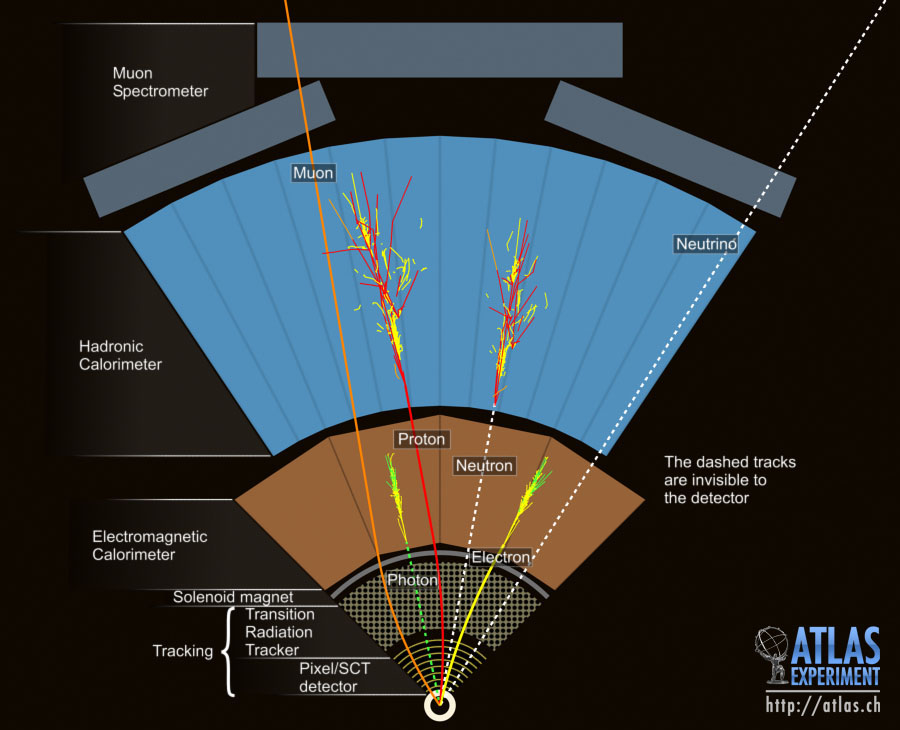
Before we move on to the section of Pileup Mitigation, it is important to understand our detector structure.<p> The ATLAS detector provides nearly full solid angle coverage around the collision point. The ATLAS tracking system is composed of a silicon pixel tracker closest to the beamline, a microstrip silicon tracker, and a straw-tube transition radiation tracker. These systems are layered radially around each other in the central region. A thin solenoid surrounding the tracker provides an axial 2T field enabling measurement of charged-particle momenta. So, when a charged particle enters the tracker, the magnetic field bends its trajectory, and the curvature of the trajectory made when it hits the silicon pixels, give us an idea about the momenta and energy of the particle.
The calorimeter is comprised of multiple subdetectors with different designs. When a particle hits the calorimeter, it deposits all its energy into the respective calorimeter section, which can be used for out analysis later. The calorimeter is comprised of two parts: ahigh granularity liquid argon (LAr) electromagnetic calorimeter system includes separate barrel, endcap, and forward subsystems, and The tile hadronic calorimeter which is composed of scintillator tiles and iron absorbers. The electromagnetic calorimeter measures energy deposits from all charged particles, whereas the hadronic calorimeter measures the energy deposits from the hadrons. The final layer is a toroid muon spectrometer (MS) that tracks muons, which are so energetic that they can survive till they reach the muon spectrometer,which is the end of the journey of any particle inside these detectors (ATLAS and CMS) . Generally, we use jets having $|\mathrm{\eta <!--\; \eta \; -->}|<2.8$ such that they are fully contained within the barrel and endcap calorimeter systems.</p>

Now, once we are done with understanding detetctor structure of ATLAS, we’ll head towards what is pileup, and how do we get rid of them. There are many p-p collisions taking place simultaneously, and within small interval of time at the Large Hadron Collider, so as to get more and more data. But multiple interactions in the same bunch crossings, and multiple bunch crossings within small time interval increases pileup. 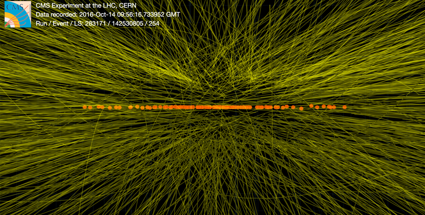Pile-up contributes to the detector signals from the collision environment, and is especially important for higher-intensity operations of the LHC. The figure below represents a typical LHC event. Each blob that we see is a reconstructed primary vertex (‘point of collision of two protons’). However each of them is not a hard scatter (deep inelastic collisions with high energy) vertex.


Hence, pileup can be of two major types:

• In Time pileup (IT): This contribution arises from the additional proton–proton (pp) collisions occurring in the same bunch crossing as the hard-scatter interaction (deep inelastic collisions with high energy).
• Out Of Time pileup (OOT): This is the pile-up from signal remnants in the ATLAS calorimeters from the energy deposits in other bunch crossings.

While pileup directly cannot be measured, it can be correlated to many directly measurable quantities, such as average number of collisions per bunch crossing ($\mathrm{\mu <!--\; \mu \; -->}$), or The observed number of collisions in a single event ($N{PV}_{}$), also known as Number of primary Vertices. Since in time pileup arise from simultaneous collisions in one buch crossing, NPV can be thought as a measure of IT. On the other hand Out of time pileups arise from remenants of signal in subsequent or previous collisions, $\mathrm{\mu <!--\; \mu \; -->}$ can be thought of as a measure of OOT pileup. Now, at this point a question might bug us that why should previous/subsequent collisions matter? It is if detector readout time is larger than the space between subsequent bunch crossings, previous, or subsequent events can overlap with current events , hence giving a wrong reconstruction. Generally, calorimeters have a longer readout, but the tracking systems have a shorter readout time.

Now, that we understand what are pileups and what are the parameters that can enable us to mitigate pileup, it is important to note that first we need to build inputs for jet reconstruction, then subtract the pileup contributions from them, and then go for final steps of callibrating these jets.

Building inputs to jet Reconstruction

So, in a detector, jets are a complex mixture of visible signals. Individual charged particles (which comprise of ~2/3 rd of the jets) appear in the tracker, wheras Charged and neutral particles (~1/3rd of the jets) appear together (but not distinguishable) in the calorimeter. So, calorimeter energy deposit is the key to jet reconstruction. But the calorimeter is succeptible to a lot of pileup as we saw previously.This means that we need to design some calorimeter objects in order to reduce pileup effects, within limits.

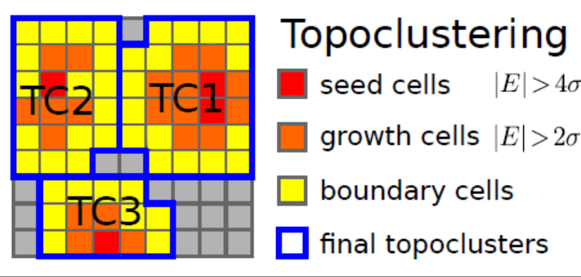Clusters of calorimeter energy are classic objects for Jet Reconstruction! We divide the calorimeter into segments. The lateral and longitudinal segmentation of the calorimeters permits three-dimensional reconstruction of particle showers, implemented in the topological clustering algorithm. Topo-clusters of calorimeter cells are seeded by cells whose absolute energy measurements |E| exceed the expected noise by four times its standard deviation. The expected noise includes both electronic noise and the average contribution from pile-up, which depends on the run conditions. The topo-clusters are then expanded both laterally and longitudinally in two steps, first by iteratively adding all adjacent cells with absolute energies two standard deviations above noise, and finally adding all cells neighbouring the previous set, just to catch the tail of the distributions. Formation of calorimeter topocluster reduces pileup to certain dergree. Nonetheless, pileup still impacts clusters. Eg: If pileup and hard scatter directly overlap, their energies are combined, changing the measured cluster energy. Also pileup can create separate topoclusters. Now these topoclusters can be used as objects for jet reconstruction, but as we saw that comes with its own problems. So, we need to do better!

So, what about tracks? Do they give us proper jet reconstruction? Althought tracks are “inherently” pileup stable, tracks give an idea about only ~2/3rd of the jet energy. The other thing is that tracks can give precise idea about energy and momentum of a charged particle only at low p_T. This is because, at high p_T, the ability to measure track curvature degrades.

Summarizing: Calo clusters are good objects for reconstruction at high energies, but at low energies they have significant pileup contributions. Tracks on the other hand can measure low energy jets quite well, but this degrades as the jet p_T increases. Hence, neither tracks, nor calo clusters can form a good reconstruction object. So then what if we combine the information from both these, and consider information from mixtures of tracks and calorimeter clusters to reconnstruct our jets? This requires matching tracks to clusters so we don’t double-count energy. Once we have matched track(s) to a cluster, we check if their measurements are consistent. If they are consistent, the cluster likely corresponds to only charged particle(s), else the cluster likely corresponds to overlapping charged and neutral particles. This process is typically called “particle flow” or (PFlow). Once again particle flow is a very detector-specifc algorithm, and each collaboration has their own algorithm, but the general idea and approach follows the above mentality. The figure below beautifully illustrates the entire PFlow algorithm:

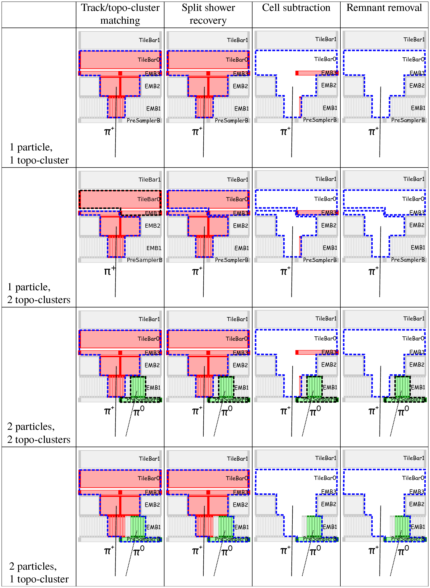Charged hadrons are identified by linking the track to one or more calorimeter clusters, while photons and neutral hadrons are in general identified by calorimeter clusters that are not linked to the track. Electrons are identified by linking the track and the cluster in the electromagnetic calorimeter, without any signal left in the hadronic calorimeter, while muons are identified as a track in the tracker detector that is linked with the corresponding track in the muon stations. A better description of particle flow is presented in this CMS paper. Now, the anti-k_T algorithm (radius parameter R = 0.4) clusters all the particles reconstructed from PFlow algorithm (PFlow jets), or the sum of the ECAL and HCAL energies deposited in the calorimeter towers (Calo jets), or all stable particles produced by the event generator excluding neutrinos (Ref jets).