Supersymmetry in ATLAS
My journey to ATLAS-2021
Getting an internship in ATLAS, one of the 4 major detectors of the Large Hadron collider (LHC), CERN was like a dream come true. The year of 2020, I applied for a project position at the University of Geneva for the summer of 2021, and fortunately got selected! I started my work from the December of 2020.
In this section I'll keep appending basically all of the Analysis techniques and methods I learn and perform for the entire duration of the project :)
R-Parity Violation Supersymmetry Analysis in ATLAS
I have discussed about Supersymmetry and R-parity in the post What’s SUSY all about?. Here I’ll discuss about the analysis work and strategies that I am learning and following for this ATLAS project of 2020-2021 that is based on Gluino R-parity violation coupling.
The signal model
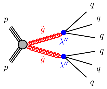 This is our signal model, also known as the 6-jet model. The feynman diagram adjoining clearly specifies that there is a
gluino pair production via R-parity conservation coupling, since a Standard model particle must have produced a pair of SUSY particle. Each of these gluinos now decay into a three quarks via R-paity
violation coupling. So, in each event, there are six quarks produced, that hadronize to produce jets (which are basically spray of particles that hit the detector).
This is our signal model, also known as the 6-jet model. The feynman diagram adjoining clearly specifies that there is a
gluino pair production via R-parity conservation coupling, since a Standard model particle must have produced a pair of SUSY particle. Each of these gluinos now decay into a three quarks via R-paity
violation coupling. So, in each event, there are six quarks produced, that hadronize to produce jets (which are basically spray of particles that hit the detector).
Why did we traget gluino pair production?
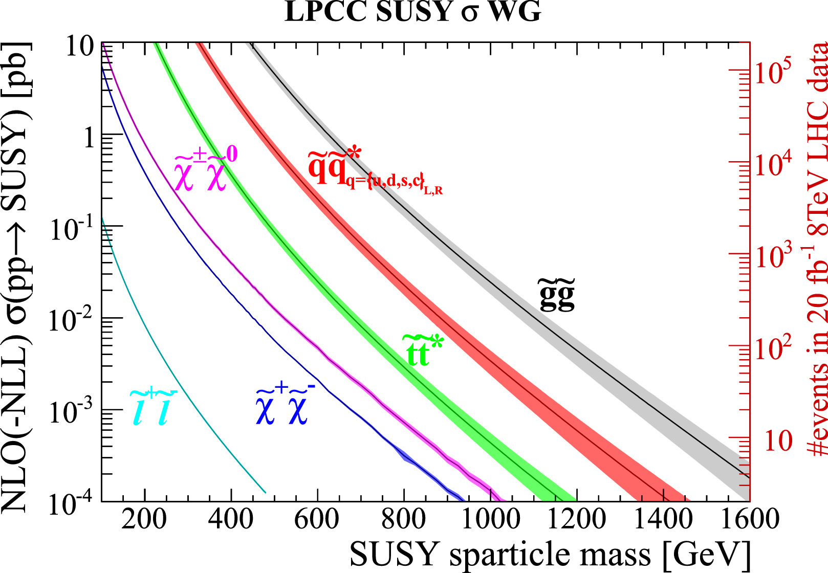 Production cross-sections (which can be considered as a ‘measure’ of probability that the process shall occur)
at the LHC are shown in the adjoining figure as a function of the sparticle mass. As expected the pair production of gluinos dominates the SUSY production for a given mass
scale, followed by the production of squarks, elecroweakinos, sleptons, and sneutrinos. This is exactly why we target gluino pair production. The fist signatures of SUSY is more probable to show up
via gluino pair production.
Production cross-sections (which can be considered as a ‘measure’ of probability that the process shall occur)
at the LHC are shown in the adjoining figure as a function of the sparticle mass. As expected the pair production of gluinos dominates the SUSY production for a given mass
scale, followed by the production of squarks, elecroweakinos, sleptons, and sneutrinos. This is exactly why we target gluino pair production. The fist signatures of SUSY is more probable to show up
via gluino pair production.
A valid question to ask is why didn't we observe a SUSY event so far? The answer to this is, lack of statistics! Supersymmetry processes are very rare, they occur with much lower crossection than the Standard Model processes, hence small statistics ensures masking of the signal (in our case any SUSY process) by the much more probable background processes (the Standard Model Processes).
Cut and Count Analysis
.png) This is the simplest and most straight-forward method to analyse the data. The basic idea behind cut and count analysis is we define an optimized signal region, where the signal is more abundant with respect to the background in terms of number of events. These optimized cuts over on the given set of variables define the signal region. By 'optimization', we generally mean a specific metric which reaches its optimum value, when such cuts are apllied in a parameter space. In order to understand it better, lets consider an example. Say we have n variables in which we wish to apply a cut to define our signal region apart from the background. If we apply a cut xi, where i=0,1,2,...n on all these n variables and calculate the optimum value of the metric f(k; xi) in this n-dimensional phase space. Here in the definition of f, k is a set of parameters. The best cut is the one that takes the metric function to its global optima. Hence, our problem of Signal Region definition boils down to finding the cuts that maximizes the value of the metric function f.
This is the simplest and most straight-forward method to analyse the data. The basic idea behind cut and count analysis is we define an optimized signal region, where the signal is more abundant with respect to the background in terms of number of events. These optimized cuts over on the given set of variables define the signal region. By 'optimization', we generally mean a specific metric which reaches its optimum value, when such cuts are apllied in a parameter space. In order to understand it better, lets consider an example. Say we have n variables in which we wish to apply a cut to define our signal region apart from the background. If we apply a cut xi, where i=0,1,2,...n on all these n variables and calculate the optimum value of the metric f(k; xi) in this n-dimensional phase space. Here in the definition of f, k is a set of parameters. The best cut is the one that takes the metric function to its global optima. Hence, our problem of Signal Region definition boils down to finding the cuts that maximizes the value of the metric function f.
The choice of the metric varies from analysis to analysis. Eg: We can choose statistical significance as defined here in this ATLAS Note. This might look quite simple, but there are quite some challenges to this. Firstly, we need to choose the right and best subsets of variables that goes into the phase space, and need to understand their correlations and each of their impact on the statistical significance (in general the metric function). Secondly and most importantly, optimization codes take a lot of time to give proper results, and initial parameter definitions (k) might lead to false trapping into some local optima, instead of a global optima. However, cut and count analysis can in general be used as a complementary approach with respect to machine learning and can be thought as to stand as a bechmark to more complicated analysis. With this we head on to understand what are the background processes we have, and whether there are some other ways to estimate the signal leaving behind most of the background contributions.
Backgrounds for our signal model?
Our signal model concerns Gluino pair production decaying via R-parity violation coupling in all hadronic final states. So, the background must contain those processes that have all hadronic final states too. The first and the most important background for this is: QCD Multijet Background, since at a hadron collider the production of multijets through QCD interaction is the highest cross-section SM process. The other fairy important backgrounds involve events, single top, and W/Z + jets.
When we model a background we generally rely on Monte Carlo simulations. But with QCD it is harder, because the processes have huge cross sections so no matter how much CPU we put at work to simulate the events, we almost always end up with too few good events to do a proper modeling job. But this is not the case for other major backgrounds, like the once discussed above. So how do we go with modelling our QCD background?
Data Driven Background Estimation
One solution to the problem that I raised in the previous section is what is popularly known as “Data Driven Background Estimation”. What this means is that we estimate the background from the data itself, without relying on our Monte Carlo, although often these estimates also use some simulation-based information. Now at first it might seem to be very weird, as in how do we know if our data contains signal or not alongside backgroud? There are many types of data driven estimate, and the process is quite subjective to which method we are using.
The ABCD method of background estimation
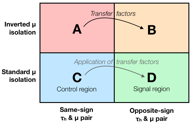 The main idea behind the ABCD method is illustrated in the diagram here. In order to find the background estimate in the signal region D, we estimate the background in a relatively signal free region called the control region C. But usually there can be some differences in the selection efficiency for the background process between regions C and D. To account for these differences, the estimate obtained in region C is corrected by so-called transfer factors. This transfer factor can be calculated from the data, as well as by the use of some Monte Carlo. The former is a fully data driven estimate, while the later is dependent on simulation parameters, hence is more prone to risk that the results are incorrect due to some incorrect model or assumption used in the simulations. Lets understand this in a bit more detail.
- The signal region:It is the region in the region in our phase space that is defined by the selections we have made for our analysis. Eg: Triggers, other offline selection, etc.
- The control region:The conrol region is defined usually by modifying the cuts w.r.t the selections we made to define our signal region. These are similar in some aspects to the signal region, but are actually signal depleated (enough statistics must be there!)
Estimating QCD Multijet Background in the Control Region
It is possible that the in the defined control region we donot just have the background process, whose shape we are trying to determine. Our data is a mixture of different processes. So, in order to ensure that we are just accounting for QCD multijet processes, we need to subtract the contribution of other major background processes from the data. Luckily, we know how to estimate all the other relevant background processes – from simulation!
The Transfer Factor
Now, that we have already estimated our QCD Multijet background we chave to figure out how to normalize it. What do I mean by normalisation here? It so occurs that the selection efficiencies of each background process most likely would not be identical in the control and the signal regions. Hence, we need to correct this. This correction is done using additional event weights, which we call here the transfer factor. In the simplest case, if the shape of the distribution of the background process is correct (same as that in signal region region D), what we can do is just normalize the events by scaling. So our transfer factor is a single number in this case, and we can weight all our events in our background estimate by this single weight.
However, usually the transfer factor depends on several variables, so we need to apply different weights to different events.
Now, a question might crop in how do we actually determine this transfer factor? The answer is, we use two more control regions for that (See A, and B in the diagram above). Here the idea is quite simple: We define A, and B by the same cuts that we applied for defining regions C and D. Thus, if we parametrize the change of our background from A to B with transfer factors, these same factors should correctly describe the difference between C and D.
So, lets say for a simple transfer factor, defined to be the fraction of event yield TF = NB/NA. Thus, it means that the number of events in the signal region D can be estimated as: ND = TF.NC= (NB/NA).NC. Now, if we want to understand the dependence of this transfer factor on different variables, we can do this with histograms so that this formula holds for each single histogram bin. With multiple variables, we have two ways to do that: Either we can use multi-dimensional histograms or just a set of one-dimensional histograms with varied selections so that we sample all the other variables that we want. It might seem a bit unclear at this stage, as the way these selections are made to define our control regions, and the variables that determine the transfer factor varry for different analysis. We can take a look at what we can do with our analysis in a future discussion, since it is still an ongoing analysis, and I cannot reveal these internal results in a public platform :)
I promise to update the material in here once the analysis is complete and the results are out in public!
But untill then lets head on to something that is really important to understand. How can we convince ourselves that our background estimation method works and gives us a good estimate? We'll take a look into this in the next section.
Validation of the Background Estimate
One way to get some confidence is to define additional signal-free validation region, again by changing some cut(s) in the analysis, then split it into the four regions A, B, C, and D in the same way as in the original analysis, and check that the background estimate agrees with data. Then we know that the method works at least in the validation region. If we look at several validation regions “around” our signal region, we can gain even more confidence in our method.
Another common approach is to use 'pseudo-data', i.e. replace the real data with a sum of simulated samples, including the background we want to estimate with ABCD such as QCD. Then we can check that the background estimation method reproduces the correct results, because this time we know the “true” background composition of our pseudo-data. This simulated pseudo-data can also have some simulated signal included in the mix, so we can check that the signal doesn’t accidentally get absorbed into our background estimate.
Updates from recent ATLAS and CMS papers on data driven methods
- Jet Counting Method: 8TeV ATLAS
- Jet Mass Template Method: 13TeV ATLAS
- Two Hemisphere Method: Paper ;
Poster
- Fit Function: CMS- Dalitz Variable Paper